Land-Use Analysis

Land-use methods aggregate data features (shops, parks, building attributes) over the network from each node. Distance decay controls how they weight nearby versus distant features, so both topics are covered on this page.

How distances to data features are measured

Several cityseer methods aggregate data over the network and need the distance from each network node to each data feature: land-use accessibility, mixed-use diversity, statistical aggregations, and the demand and origin-destination models. A data feature may be a point, a line, or a polygon. The distance is measured along the streets, with a final step off the network to the feature itself. It is computed in two phases: assignment, done once when the data layer is built, and aggregation, done from every source node as the shortest paths are computed.

Assignment: binding a feature to the network

Assignment determines which street each feature is measured from and records an offset for the match. A point is matched to its closest adjacent street. A line or polygon is more diffuse, so its closest street cannot reliably be taken as the point of access; it is matched to every street directly surrounding it instead. The offset has two parts, added together: an along-street distance and a perpendicular setback s, the gap between the feature and the street. The streets are selected in this order:

1. A spatial index returns several nearby candidate streets. For a point, these are the nearest by distance. For a line or polygon, the index returns every street whose bounding box lies within max_netw_assign_dist.
2. The true distance from the feature to each candidate is measured, and any candidate beyond max_netw_assign_dist (default 100m) is dropped.
3. The surviving candidates are sorted, nearest first.
4. Each candidate is tested in that order. A street that lies inside or touches the feature is accepted at once. Otherwise the connector, the straight line from the feature’s nearest point to the street, must not cross a barrier (from barriers_gdf) or another street; this keeps a feature from binding across a road a pedestrian would have to cross. A candidate whose connector crosses either is skipped.
5. A point keeps only the first candidate that passes. A line or polygon keeps all that pass.

A feature with no valid street within max_netw_assign_dist is left unassigned and takes no part in any aggregation.

Aggregation: measuring from each node

From each source node, a shortest-path traversal (or a simplest-path traversal, with angular=True) gives the network distance to every reachable node. The distance to a feature is the network distance to its assigned street plus the offset recorded during assignment, and it depends on the direction of approach: a feature can be reached from either end of its street, and the offset that applies is set by the end the route arrives through. cc_{category}_nearest_max_{distance} reports the nearest such distance for a category; accessibility counts and weighted statistics use the same distance to decide threshold membership and decay weight.

How the offset is recorded, and how the direction of approach is resolved, depends on the graph representation.

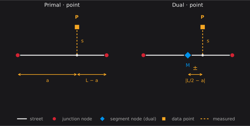The final distance depends on the direction the route approaches from. Amber marks the point and its measured offset; the street is drawn the same in both panels. Primal (left): the point attaches to both junction nodes; the distance through an end is the network distance to that node, plus the along-street part (a from one end, L − a from the other), plus the setback s, and the direction of approach settles which end applies. Dual (right): the point attaches to one segment node at the midpoint M; the along-street term |L/2 − a| is added or subtracted according to which end the route enters through, plus s.

Primal: both ends of the street. On a primal graph the point attaches to both ends of its nearest street, with the along-street distance to its projection recorded at each: a from one end, L − a from the other, where L is the segment length. The route arrives through the nearer end, and the distance is the network distance to that end, plus that end’s along-street part, plus the setback s. The direction of approach sets which end is nearer, and so which distance applies.

Dual: the segment’s centre point. On a dual graph the point cannot attach to two ends, because each junction is shared by several streets. It attaches instead to one node, the segment’s centre point M. Depending on the direction of approach, the along-street offset |L/2 − a| is added to or subtracted from the network distance, and the setback s is added. This single-segment binding applies from version 5.6 onward.

Deduplication. A single real-world feature is sometimes recorded as several points; a building, for instance, may have a separate point for each entrance. Give those points a common value and pass it as data_id_col to mark them as one feature. During aggregation only the closest of them is counted from each source node, so the building is measured to its nearest entrance.

Lines and polygons. If more precise alignment is wanted, a point data type can be used instead, placed at the actual entrance to the building or feature (figure below). Where there are several entrances, denote each with its own point but give them a shared data_id_col, so the algorithm counts only the distance to the nearest and does not double count.

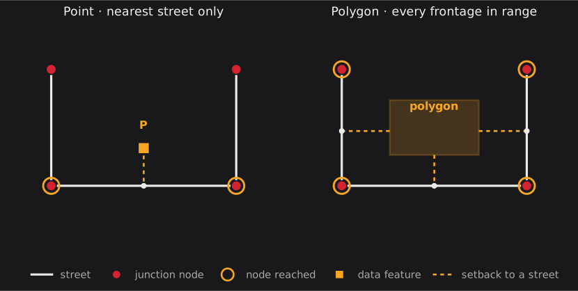On a primal graph. Left: the point reaches only its nearest street, so only that street’s two junction nodes are reached. Right: the polygon faces three streets within range and binds to each, so every one of those streets’ nodes can reach it.

Two parameters control assignment on any of these methods. max_netw_assign_dist sets how far a feature may sit from a street before it is dropped. data_id_col names a column holding a unique identifier for the original feature that several points represent. Points sharing that identifier are treated as one feature, so only the nearest is counted.

cn.compute_accessibilities(
    data_gdf=data_gdf,
    landuse_column_label="category",
    accessibility_keys=["park"],
    distances=[800],
    max_netw_assign_dist=100,
    data_id_col="feature_id",
)

Decay functions

Distance decay controls how the weight given to a feature, or a metric contribution, decreases with distance from an analysis point. For centrality, decay is built into the metric expressions (e.g. the default "exp(-4 * p)" closeness and betweenness metrics described on the Centrality page). For land-use methods (compute_accessibilities, compute_mixed_uses, compute_stats), an optional decay_fn parameter accepts a string expression using a variable p that ranges from 0 at the source to 1 at the distance cutoff (p = network_distance / max_distance). The cityseer.decay module provides helper functions that return pre-built expression strings for common decay shapes.

How decay weighting works

A decay function maps normalised progress p to a weight. p = 0 at the analysis node (the source) and p = 1 at the distance (or time) cutoff, so p = network_distance / threshold. The function is evaluated once per reached element, for every reachable node in a centrality calculation, or every reachable data feature in a land-use calculation, and the resulting weight scales that element’s contribution to the metric (a count, a numerical value, or a diversity contribution).

A few properties are worth understanding:

• Per-threshold normalisation. When several distances are requested, p is recomputed against each threshold independently. The same physical point therefore has a larger p (and so less weight under a decaying function) at a short threshold than at a long one, keeping every catchment internally consistent.
• Clamping (land-use only). Land-use decay output is clamped to [0, 1], so an expression can never produce negative or amplifying weights. Centrality expressions are not clamped, because they are general metric formulas (e.g. 1/c) rather than weights.
• Flat by default for land-use. With the CityNetwork default of "1", every reachable point contributes a weight of 1, i.e. a plain unweighted count or sum within the threshold (see Default decay behaviour for the lower-level layers default).
• Decay vs. metric. In centrality the decay is simply one possible metric expression (the default "exp(-4 * p)" decay/betweenness_decay columns). In the land-use methods the decay is a separate decay_fn that multiplies whatever is being aggregated.

When to use each preset

Preset	Helper	When to use
Exponential	decay.exponential()	Pedestrian catchments where nearby destinations count far more than distant ones. Default for centrality.
Linear	decay.linear()	Uniform distance penalty with no abrupt boundary.
Flat	decay.flat()	Simple counts within a threshold, with no distance weighting. Default for accessibility and stats.
Gaussian	decay.gaussian(peak, cutoff, std)	Use cases where peak relevance sits at some distance from the source, not immediately adjacent.
Logistic	decay.logistic(midpoint, cutoff)	Catchment boundaries with a gradual transition rather than a hard cutoff.

Code examples

Centrality metrics are specified as {name: expression} dicts using variables c (cost) and p (normalised progress). Land-use methods use decay_fn with the p variable:

from cityseer import decay

# Centrality: custom closeness metric using c (cost in metres)
cn.centrality_shortest(
    distances=[800],
    closeness={"gravity": "exp(-0.005 * c)", "harmonic": "1/c"},
)

# Gaussian decay for land-use stats
cn.compute_stats(
    data_gdf=prices_gdf,
    stats_column_labels=["price"],
    distances=[1200],
    decay_fn=decay.gaussian(peak=400, cutoff=1200, std=150),
)

Default decay behaviour

• Centrality (centrality_shortest): default closeness includes "decay": "exp(-4 * p)" and default betweenness includes "betweenness_decay": "exp(-4 * p)".
• Accessibility and stats (compute_accessibilities, compute_mixed_uses, compute_stats): the CityNetwork methods default to "1" (flat, no distance weighting); pass a decay expression explicitly for distance-weighted aggregations. The lower-level layers functions retain the legacy default when decay_fn is omitted, producing both an unweighted (_nw) and a decay-weighted (_wt) column; pass a single expression to compute one unsuffixed column instead.

Multiple decays in one traversal

The expensive part of a land-use computation is the network traversal from every node; applying a decay weight to the reachable features is cheap by comparison. So instead of calling a method once per decay shape, repeating the traversal each time, the land-use methods (compute_accessibilities, compute_mixed_uses, compute_stats) let decay_fn be a {label: expression} dict and compute every decay variant in a single shared traversal.

• Input. decay_fn may be a single expression string, None (flat, the default), or a {label: expression} dict.
• Output naming. Each label is appended to that variant’s output columns: decay_fn={"grav": ..., "raw": ...} yields cc_retail_grav_800, cc_retail_raw_800, and so on. A plain string or None adds no suffix, so existing column names, and their values, are unchanged. The dict form is therefore purely additive and backwards compatible.
• When to use it. Whenever you want the same features summarised under more than one distance weighting: a gravity-weighted and a plain count of the same amenity; or several catchment shapes (exponential, Gaussian, flat) for a sensitivity analysis. A pipeline that previously made N calls collapses to one.

# gravity-weighted AND plain-count accessibility to retail, in one pass
cn.compute_accessibilities(
    data_gdf=landuses_gdf,
    landuse_column_label="category",
    accessibility_keys=["retail"],
    distances=[800],
    decay_fn={"grav": decay.gaussian(peak=200, cutoff=800, std=150), "raw": decay.flat()},
)
print(cn.nodes_gdf[["cc_retail_grav_800", "cc_retail_raw_800"]])

This mirrors how centrality_shortest accepts a {name: expression} dict of metrics evaluated in a single traversal. Each labelled variant produces the method’s full set of output columns. One caveat for compute_mixed_uses: only the Hill measures are distance-weighted (they use branch-distance weighting), so Shannon and Gini are computed from raw category counts and will be identical across labels.

Expression syntax

Centrality expressions use two variables: c (raw cost) and p (normalised progress, c / threshold). Land-use decay expressions use p only. Both are evaluated by the same runtime expression engine, which supports the operators +, -, *, /, and ^ (power), the functions exp, ln, log10, sqrt, abs, sin, cos, tan, floor, ceil, and round, and the constants PI and E. ** is not accepted (write ^), min and max are not available, and unary minus binds tighter than the power operator, so write -(p^2) rather than -p^2 when the square should be negated. Land-use decay output is clamped to [0, 1]; centrality expressions are not clamped.

The centrality postprocess parameter is the one exception: it is evaluated in Python over previously computed metric columns and supports only +, -, *, /, and ** (power), with no functions; see Custom metrics. See the cityseer.decay API reference for full details.

Land-use methods

cityseer computes land-use and statistical aggregations at the same node locations used for centrality. Because the results share a common spatial index, you can directly compare how well-connected a location is (centrality) with what amenities are reachable from it (accessibility). All land-use methods accept an angular=True parameter for simplest-path routing (CityNetwork handles the required dual graph automatically).

Accessibility

Accessibility answers a resident’s question: from here, how much of a given kind of place can I reach on foot, and how far is the nearest one? A node with high retail accessibility sits within reach of many shops; a large nearest_max distance means the closest one is far away.

compute_accessibilities measures how many instances of each specified land-use category are reachable from every network node, and how far away the nearest instance is. For each category key and distance threshold it writes two kinds of column:

• cc_{category}_{distance}: the (optionally decay-weighted) count of reachable instances of that category within the threshold. With the default flat decay this is a plain count; with a decaying decay_fn it becomes a distance-weighted “gravity” accessibility.
• cc_{category}_nearest_max_{distance}: the network distance to the nearest instance of that category. This is written only at the largest threshold, since the nearest distance does not depend on the catchment size.

Pass decay_fn to weight counts by distance, including the {label: expression} dict form to produce several weightings at once (see Multiple decays in one traversal). The angular=True parameter enables simplest-path routing.

The column names above reflect the CityNetwork method, whose default decay_fn of "1" yields a plain count. When decay_fn is omitted on the lower-level layers.compute_accessibilities function, the legacy default writes both an unweighted cc_{category}_{distance}_nw and a decay-weighted cc_{category}_{distance}_wt column; passing a single expression produces one unsuffixed column.

cn.compute_accessibilities(
    data_gdf=landuses_gdf,
    landuse_column_label="category",
    accessibility_keys=["retail", "cafe", "park"],
    distances=[400, 800],
)
print(cn.nodes_gdf["cc_retail_800"])           # count within 800m
print(cn.nodes_gdf["cc_park_nearest_max_800"]) # nearest distance to park

See the OSM Accessibility recipe.

Mixed-use diversity

Mixed-use diversity measures how varied the surroundings are, beyond a plain count. A street where all ten premises are cafes is less mixed than one where the ten are spread across cafes, shops, a school, and a clinic, though both have the same number of premises. Hill numbers express this as an effective number of land-use types: the count you would have if every type present were equally common.

compute_mixed_uses measures this diversity from every network node. Hill numbers are computed by default (compute_hill=True); Shannon and Gini-Simpson indices are available via the compute_shannon and compute_gini flags. The order q sets how much the balance of common versus rare types counts:

• Hill q=0 (cc_hill_q0_{d}) counts how many different land-use types are present, ignoring their balance (species richness). Best with many fine-grained categories.
• Hill q=1 (cc_hill_q1_{d}) reflects both how many types are present and how evenly they are represented (the exponential of Shannon entropy).
• Hill q=2 (cc_hill_q2_{d}) is dominated by the most common types and largely discounts rare ones (the inverse of the Simpson concentration index). Best with broad categories where the balance of dominant types matters most.

The Hill measures are distance-weighted through a branch-distance form, so a decay_fn shapes how strongly nearer instances count. Shannon (cc_shannon_{d}) and Gini (cc_gini_{d}) are computed from raw category counts and are not affected by decay_fn.

See the Mixed Uses recipe.

Statistical aggregations

Statistical aggregation summarises a numeric attribute of the features around each node, measured over the network rather than a straight-line buffer. Given a column such as building height, dwelling price, or plot area, it reports what you would meet within a walk of each street: the mean value, the total, the spread, and so on. The summary uses the same distance decay as the other methods, so nearer features can count for more than distant ones.

compute_stats computes these statistics for one or more numerical columns. For each input column and distance threshold it writes eight measures, named cc_{column}_{measure}_{distance}:

Measure	Column suffix	Notes
Sum	_sum	Decay-weighted sum of values.
Mean	_mean	Decay-weighted mean.
Count	_count	Sum of decay weights (a plain count under flat decay).
Variance	_var	Decay-weighted variance.
Median	_median	Weighted median.
MAD	_mad	Weighted median absolute deviation.
Max / Min	_max / _min	Extremes of reachable values (not affected by decay_fn).

Pass a list of stats_column_labels to summarise several columns in one call, and a decay_fn to weight each value by distance, including the {label: expression} dict form for multiple weightings in a single traversal. By default all eight measures are produced; pass measures=[...] (any subset of the suffixes above) to compute only the ones you need. This keeps the output GeoDataFrame smaller and skips the weighted median/MAD sort when neither is requested.

cn.compute_stats(
    data_gdf=prices_gdf,
    stats_column_labels=["price"],
    distances=[1200],
    decay_fn=decay.gaussian(peak=400, cutoff=1200, std=150),
)
print(cn.nodes_gdf["cc_price_mean_1200"])

See the Statistical Aggregations recipe.