Centrality

Centrality metrics quantify the structural importance of each location in the street network. cityseer computes multiple centrality measures simultaneously for any combination of distance thresholds in a single pass.

Expression-based metrics

Metrics are defined as {name: expression} dictionaries using two variables:

• c (cost): the raw routing cost to each reached node. For shortest paths, c is the metric distance in metres. For simplest paths, c is the cumulative angular change in degrees.
• p (progress): normalised progress from 0 at the source to 1 at the distance threshold. For shortest paths, p = c / threshold. For simplest paths, p = elapsed_time / max_time.

Metrics fall into four categories:

Category	Role	Example
Closeness	Expression is evaluated once per reached node and summed across all reachable nodes.	{"harmonic": "1/c"} accumulates $\sum_j 1/c_j$
Betweenness	Expression weights the contribution of each destination during Brandes backpropagation.	{"betweenness": "1"} counts paths equally
Cycles	Boolean flag; computes the circuit rank of the locally reachable subgraph (shortest-path only).	cycles=True
Postprocess	Derives new columns from previously computed metrics using simple arithmetic (+, -, *, /, **).	{"hillier": "density**2 / farness"}

Pass None to use the defaults for a category, or {} to skip it entirely. The default sets described below are those of the lower-level metrics.networks functions; the CityNetwork methods default to a leaner set, a single harmonic closeness and a single unweighted betweenness, with cycles and postprocess off. Pass the expression dicts explicitly to compute any of the fuller set.

Shortest-path centrality

centrality_shortest (or centrality_shortest in the lower-level API) computes the following default metrics for each distance threshold d. In the formulas below, the sum is over all nodes $j$ reachable within $d$, $c_j$ is the shortest-path distance in metres to node $j$, and $p_j = c_j / d$.

Default closeness (pass closeness=None or omit):

Column	Expression	Formula	Description
cc_density_{d}	"1"	$\sum_j 1$	Count of nodes reachable within distance $d$. A simple measure of local connectivity.
cc_farness_{d}	"c"	$\sum_j c_j$	Sum of metric distances to all reachable nodes. Lower values indicate better average proximity.
cc_harmonic_{d}	"1/c"	$\sum_j 1 / c_j$	Harmonic closeness: sum of inverse distances. Higher values indicate better proximity. Unlike standard closeness, harmonic closeness handles distance-bounded analysis correctly because unreachable nodes contribute 0 rather than distorting the average.
cc_decay_{d}	"exp(-4 * p)"	$\sum_j e^{-4 p_j}$	Exponential decay-weighted closeness. Nearby nodes contribute most; at the distance threshold ($p = 1$), weight drops to $e^{-4} \approx 1.8\%$. This is the continuous equivalent of the historical $\beta$-weighted metric.

Default betweenness (pass betweenness=None or omit):

Column	Expression	Formula	Description
cc_betweenness_{d}	"1"	$\sum_{s,t} \sigma_{st}(v) / \sigma_{st}$	Unweighted betweenness: for each origin–destination pair $(s, t)$, counts the fraction of shortest paths that pass through node $v$. High values indicate through-movement potential.
cc_betweenness_decay_{d}	"exp(-4 * p)"	$\sum_{s,t} e^{-4 p_t} \cdot \sigma_{st}(v) / \sigma_{st}$	Decay-weighted betweenness: each pair’s contribution is downweighted by the exponential decay applied to the destination’s normalised distance $p_t$. Paths to distant destinations count less.

Default postprocess (pass postprocess=None or omit):

Column	Expression	Formula	Description
cc_hillier_{d}	"density**2 / farness"	$n^2 / \sum_j c_j$	Hillier normalisation: rewards locations that are both well-connected (high density $n$) and proximate (low farness). This is the standard normalisation used in space syntax research.

Cycles (cycles=True by default):

Column	Description
cc_cycles_{d}	Circuit rank of the locally reachable subgraph: the number of independent loops ($e - n + 1$ where $e$ is edges and $n$ is nodes in the subgraph). In grid-like networks, each loop roughly corresponds to a city block; in less regular networks, it measures the redundancy of route choices.

Simplest-path centrality

centrality_simplest (or centrality_simplest in the lower-level API) computes angular centrality metrics. For simplest paths, c is the cumulative angular change in degrees (the total turning at each junction along a route) rather than metric distance. The variable p is normalised elapsed time (not angular cost), so the distance reachability budget is still metric. Note the _ang suffix on all output columns.

Default closeness (pass closeness=None or omit):

Column	Expression	Formula	Description
cc_density_{d}_ang	"1"	$\sum_j 1$	Count of nodes reachable within distance $d$ via angular routing.
cc_farness_{d}_ang	"1 + c / 90"	$\sum_j (1 + c_j / 90)$	Angular farness. The $1 + c/90$ transform maps a straight-ahead path ($0°$) to 1 and a single $90°$ turn to 2, giving a meaningful scale that avoids division-by-zero at the source. Equivalent to angular integration in space syntax.
cc_harmonic_{d}_ang	"1 / (1 + c / 90)"	$\sum_j 1 / (1 + c_j / 90)$	Angular harmonic closeness: the inverse of the farness expression. Higher values indicate better angular proximity (straighter routes to more destinations).

Default betweenness (pass betweenness=None or omit):

Column	Expression	Formula	Description
cc_betweenness_{d}_ang	"1"	$\sum_{s,t} \sigma_{st}(v) / \sigma_{st}$	Angular betweenness: fraction of simplest (minimum angular change) paths through each node. Equivalent to angular choice in space syntax.

Default postprocess (pass postprocess=None or omit):

Column	Expression	Formula	Description
cc_hillier_{d}_ang	"density**2 / farness"	$n^2 / \sum_j (1 + c_j / 90)$	Hillier normalisation for angular metrics.

Simplest-path centrality does not include decay-weighted metrics by default because angular cost is not a distance measure. Decay-weighted angular metrics can be added via custom expressions if needed.

Choosing shortest or angular

The two are not interchangeable. The right choice depends on the network’s condition as well as the research question.

Shortest-path (metric) centrality is the general-purpose choice. Metric distance is well defined regardless of how tidy the network representation is, so shortest-path measures degrade gracefully when the geometry carries noise: extra nodes, un-merged dual carriageways, or slightly misplaced junctions shift the numbers only slightly. It applies across morphologies, and it is the safer option for messier or less thoroughly cleaned networks, and for cities where physical travel distance is what governs movement.

Simplest-path (angular) centrality weights routes by cumulative turning rather than distance, following the space-syntax idea that people navigate by minimising directional complexity. On a clean, well-consolidated network, angular measures can correspond more closely with observed pedestrian and vehicular movement than metric ones. The important caveat is that angular cost is highly sensitive to the network representation. Spurious nodes, unconsolidated parallel edges, roundabouts left as rings, and noisy geometry all distort the turn angles that the measure is built from, so angular results are only trustworthy on a carefully cleaned network (see Network Cleaning). On a messy network, angular centrality can mislead, whereas shortest-path centrality stays robust.

A practical rule: shortest-path always applies. Reach for angular when the network is clean and you specifically want a route-complexity model of movement, and sanity-check the angular pattern against the metric one.

Custom metrics

To define custom metrics, pass a dictionary of {name: expression} pairs. Closeness and betweenness expressions (and decay_fn expressions elsewhere) are evaluated by the runtime expression engine: they can use the variables c and p, the operators +, -, *, /, and ^ (power), and the functions exp, ln, log10, sqrt, abs, sin, cos, tan, floor, ceil, and round, plus the constants PI and E. Note that ** is not accepted (write ^), min and max are not available, and unary minus binds tighter than the power operator, so write -(p^2) rather than -p^2 when the square should be negated.

Postprocess expressions follow different rules: they are evaluated in Python over the previously computed metric columns and support only the arithmetic operators +, -, *, /, and ** (power), with no functions. In postprocess, power is written **, not ^.

# Custom gravity model and linear-decay betweenness
cn.centrality_shortest(
    distances=[800],
    closeness={"gravity": "1 / c^2", "reach": "1"},
    betweenness={"bt_linear": "1 - p"},
    postprocess={},  # skip hillier
)

# Angular centrality with decay-weighted betweenness
cn.centrality_simplest(
    distances=[800],
    betweenness={"betweenness": "1", "bt_decay": "exp(-4 * p)"},
)

Node weights

Every node carries a weight (default 1.0). Set it on the nodes GeoDataFrame, or add a weight attribute to your NetworkX nodes before ingestion, to apply gravity-style weighting to centrality:

• Closeness weights each reachable node by its destination weight, so density becomes $\sum_j w_j$ (the sum of reachable node weights) rather than a plain count, and other closeness expressions are scaled accordingly. A node’s own weight does not rescale its own score; weighting reflects the opportunities it can reach.
• Betweenness weights each origin–destination pair by the product of its endpoint weights $w_s \cdot w_t$, the standard gravity-flow form.

The same weighting is applied identically whether or not adaptive sampling is used. With the default weights of 1.0 the results are unchanged from an unweighted analysis.

Segment-weighted centrality

segment_weighted=True is a convenience preset over the node weight mechanism above: it temporarily sets each dual-graph node’s weight to its corresponding street segment length, then restores the original weights afterwards. This means:

• Closeness metrics reflect total reachable street length rather than node counts (e.g. density becomes total metres of reachable street within the threshold).
• Betweenness weights each origin–destination pair by both endpoint segment lengths, so longer streets contribute more to betweenness flows.

This requires a dual graph representation (which CityNetwork builds automatically).

cn.centrality_shortest(distances=[800], segment_weighted=True)

Convenience wrappers

For cases where only closeness or only betweenness is needed, convenience functions skip the unused category:

• closeness_shortest / closeness_simplest: closeness only (betweenness disabled)
• betweenness_shortest / betweenness_simplest: betweenness only (closeness and cycles disabled)

Origin–destination and demand betweenness

Standard betweenness treats every node pair equally. When you have real or modelled travel flows, cityseer can route those flows instead, with betweenness_od for an explicit origin–destination matrix and betweenness_demand for a modelled, singly-constrained spatial interaction model. This has its own dedicated section: see the Origin-Destination Flows guide and the flow recipes.

Centrality recipes

• Metric Centrality from GeoDataFrame – shortest-path centrality workflow
• Angular Centrality from GeoDataFrame – simplest-path centrality workflow
• OSM Centrality – end-to-end from OpenStreetMap
• Custom Expressions – defining custom metrics, selecting only what you need, postprocess, and statistic selection
• Sampled Centrality – adaptive sampling on a large network, validated against exact results
• OD Betweenness – demand-weighted flows from a singly constrained spatial interaction model

Performance and Scale

The underlying algorithms are parallelised in Rust and scale to large networks. Computation scales with the number of edges, the number of distance thresholds, and the reachability at each threshold. Simplest-path (angular) centrality is typically faster than shortest-path because angular routing explores fewer paths. For large networks at long distance thresholds, consider adaptive sampling.

Adaptive Sampling

For large networks at long distance thresholds, cityseer offers an experimental adaptive sampling feature. Rather than using every node as a source, each node is included with its own probability derived from its measured local reach: a cheap pilot polls the network with bounded shortest-path traversals from a small sample of sources to estimate each node’s reach, and the Hoeffding inequality converts that reach into the minimum sampling rate needed to keep the approximation error within a specified tolerance. Sparse areas are sampled more heavily and dense areas less, so precision is uniform across the network. Results are corrected using inverse-probability weighting (IPW): if a node had a 25% chance of being selected as a source, its contribution is multiplied by 4 (the reciprocal of 0.25), so that the sampled subset approximates the result of using all nodes without bias.

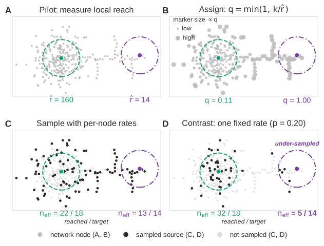The pilot measures each node’s catchment (A) and converts the measurements into per-node inclusion probabilities (B); a draw under those probabilities gives each catchment the samples it needs (C), whereas a fixed rate spending the same budget oversamples the dense core and misses most of the sparse catchment it should count in full (D).

Sampling is applied per distance threshold. For each distance, the estimated cost of properly powered sampling is compared against exact computation, and the cheaper option is selected automatically; short distances and networks with small live areas therefore run exactly, while long distances on large networks are sampled. The sampling page illustrates this decision.

The epsilon parameter controls the error tolerance. The default of 0.05 is calibrated on real networks spanning the density range, from dense metropolitan grids to a sparse suburb, so that node rankings are preserved (Spearman ρ ≥ 0.95); denser networks clear the target comfortably, while networks sparser than a typical suburb may require a tighter tolerance (see the sampling page). Both centrality_shortest and centrality_simplest support sampling. Pass sample=True to enable:

cn.centrality_shortest(
    distances=[800, 2000, 5000],
    sample=True,
)

For technical details, see the metrics.sampling documentation.